3 Position as a function of time
In the previous chapter we found the relationship between orbital position (\(\vec r\)) and true anomaly (\(\theta\)) for the two-body problem. But for any meaningful analysis of the orbital motion one would need position as a function of time. For this, we start from the conservation of angular momentum , which we can write as:
\[ h=r^2\dot \theta \]
Then,
\[ \frac{d\theta}{dt}=\frac{h}{r^2} \]
Integrating from perigee position, we get;
\[ \int_0^\theta \,d\theta=\int_{t_p}^t \frac{h}{r^2} \,dt \]
Where the true anomaly at perigee is fixed as 0, since eccentricity vector is along the perigee direction from the focus (see Figure 2.1 for explanation) and time of passing the perigee is taken as \(t_p\).
3.1 Case 1: Circular Orbits (e=0)
In case of circular orbits, \(\dot \theta\) is a constant since r is a constant. Hence,
\[ \theta (t)=\frac{h}{r^2}(t-t_p) \]
If the object in question passes perigee( because a circle is symmetric about any diameter, you can choose any radius line as the apse-line) at \(t_p=0\), and use Equation 2.9 with \(e=0\) then the equation becomes:
\[ \theta (t)=\frac{h}{\left(\frac{h^2}{\mu}\right)^2}t=\frac{\mu^2}{h^3}t \]
3.2 Case 2: Elliptical orbits (0<e<1)
Using Equation 2.9 and \(t_p=0\) ,
\[ \int_0^\theta \,d\theta=\int_{0}^t \frac{h}{\left(\frac{h^2}{\mu}\right)^2}(1+e\cos{\theta})^2 \,dt \]
\[ \int_0^t \frac{\mu^2}{h^3}\,dt=\int_0^\theta \frac{d\theta}{(1+e\cos{\theta})^2} \]
Currently we can find from integral tables that:
\[ \int_0^\theta \frac{d\theta}{(1+e\cos{\theta})^2}= \frac{1}{(1-e^2)^{3/2}}\left[2\tan^{-1}{\left(\sqrt{\frac{1-e}{1+e}}\tan{\frac{\theta}{2}}\right)}-\frac{e\sqrt{1-e^2}}{1+e\cos{\theta}}\sin{\theta}\right] \]
And therefore,
\[ \frac{\mu^2}{h^3}t=\frac{1}{(1-e^2)^{3/2}}\left[2\tan^{-1}{\left(\sqrt{\frac{1-e}{1+e}}\tan{\frac{\theta}{2}}\right)}-\frac{e\sqrt{1-e^2}}{1+e\cos{\theta}}\sin{\theta}\right] \]
We now introduce the quantity of mean anomaly, given by:
\[ M_e=(1-e)^{3/2}\frac{\mu^2}{h^3}t \tag{3.1}\]
which gives,
\[ M_e=2\tan^{-1}{\left(\sqrt{\frac{1-e}{1+e}}\tan{\frac{\theta}{2}}\right)}-\frac{e\sqrt{1-e^2}}{1+e\cos{\theta}}\sin{\theta} \tag{3.2}\]
Mean anomaly can be described of as the orbital position of a fictitious second body that moves in a circular orbit around the 1st body with the same time period as the second body in our two-body system.
\[ M_e=\frac{2\pi}{T}t \tag{3.3}\]
where \(T\) is the time period of the orbit.
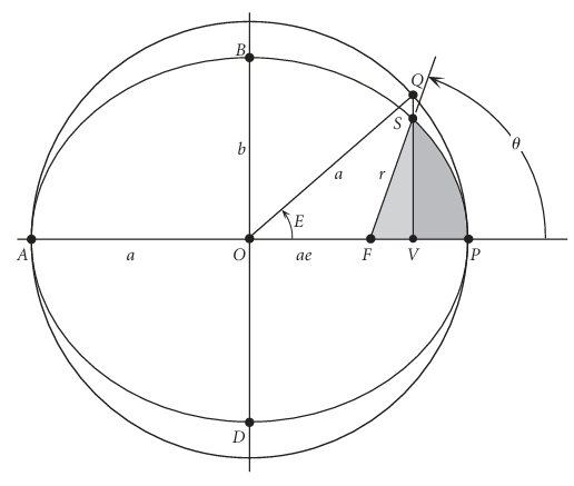
We will see that it becomes convenient to simplify Equation 3.2 by introducing an auxiliary angle \(E\) called the eccentric anomaly, which is done by circumscribing the ellipse with a concentric auxiliary circle having radius equal to the semi-major axis \(a\) of the ellipse. (Shown in Figure 3.1). Where \(S\) is the current position with true anomaly \(\theta\) and \(Q\) is the projected point onto the auxiliary circle.
From the figure, we can observe that \(\overline{OV}=a\cos E\) in terms of eccentric anomaly while \(\overline{OV}= ae + r\cos \theta\) in terms of true anomaly. Thus,
\[ a\cos E=ae + r\cos \theta \]
Using the parametric equation of ellipse Equation 1.7 with the semi-latus rectum \(p=a(1-e^2)\), we can write this as
\[ a\cos E=ae + \frac{a(1-e^2)}{1+e\cos \theta}\cos \theta \]
On simplification,
\[ \cos E = \frac{e+\cos \theta}{1+ e\cos \theta} \tag{3.4}\]
Using \(\cos^2 E + \sin^2 E=1\);
\[ \sin E= \frac{ \sqrt{1-e^2} \sin \theta}{1+e\cos \theta} \tag{3.5}\]
While using either of Equation 3.4 or Equation 3.5 is fine for obtaining \(E\) from \(\theta\), however, given a value of \(\cos E/\sin E\) between -1 and 1. there are two values of \(E \in [0,2\pi]\). To resolve the quadrant ambiguity, one is forced to check the other equation. Instead of that, we can use the following:
\[ \tan^2 \frac{E}{2} = \frac{\sin^2 \frac{E}{2}}{\cos^2 \frac{E}{2}}= \frac{1-\cos E}{1+\cos E} \]
And using Equation 3.4 on numerator and denominator,
\[ 1-\cos E=1-\frac{e+\cos \theta}{1+ e\cos \theta}=\frac{(1-e)(1-\cos \theta)}{1+ e\cos \theta} \]
\[ 1+\cos E= 1+\frac{e+\cos \theta}{1+ e\cos \theta}=\frac{(1+e)(1+\cos \theta)}{1+ e\cos \theta} \]
Therefore,
\[ \tan^2 \frac{E}{2} = \frac{1-\cos E}{1+\cos E}= \frac{(1-e)(1-\cos \theta)}{(1+e)(1+\cos \theta)}=\frac{1-e}{1+e} \tan^2 \frac{\theta}{2} \]
\[ \boxed{\tan \frac{E}{2}=\sqrt{\frac{1-e}{1+e}}\tan \frac{\theta}{2}} \tag{3.6}\]
Using Equation 3.6 and Equation 3.5 on Equation 3.2
\[ M_e=2\tan^{-1}{\left(\sqrt{\frac{1-e}{1+e}}\tan{\frac{\theta}{2}}\right)}-\frac{e\sqrt{1-e^2}}{1+e\cos{\theta}}\sin{\theta} \]
we get,
\[ \boxed{M_e= E-\sin E} \tag{3.7}\]
This is known as the Kepler’s equation.Now, given the time-period (\(T\)), eccentricity (\(e\)) and the true anomaly(\(\theta\)) position of an object in orbit, we will:
find \(E=2\tan^{-1}{\left(\sqrt{\frac{1-e}{1+e}}\tan \frac{f}{2}\right)}\)
Solve Kepler’s equation to get \(M_e\)
get the time since the previous perigee passing from Equation 3.1 .
Now looking back at history, we would see that Kepler derived this equation way before Newton formulated the principles of calculus. One could ask how he derived this relationship between two quantities that had not much of a physical significance before. This is the question that we will try to answer in the following section.
3.3 Keplerian geometrical derivation
Kepler knew from his Second Law (equal areas in equal times) that time must be proportional to the area swept out by the radius vector. Which implies,
\[ \frac{A(t)}{\pi ab}=\frac{t}{T} \tag{3.8}\]
3.3.1 Kepler’s reason for eccentric anomaly
It’s difficult to measure the swept area directly in an ellipse. Instead, Kepler mapped point \(P\) on the ellipse to point \(Q\) on the auxiliary circle. He then used the circle’s geometry to calculate areas. So if we can express \(A(E)\) as a function of \(E\), we can connect time \(t\) to its position.
3.3.2 Calculation of the swept out area
In Figure 3.1, the area swept out by the radius vector \(FP\) from periapsis \(A\) to the body \(P\) (the shaded region \(AFP\)) is what Kepler’s Second Law refers to. This area \(A(E)\) can be obtained by relating it to easier-to-compute parts:
Sector \(AOQ\) in the circle: Its area is \(\tfrac{1}{2}a^2 E\).
Ellipse correction: Since the ellipse is “squashed” vertically by a factor \(b/a\), the corresponding ellipse area is scaled: \(\tfrac{1}{2}ab E\).
Shift from center \(O\) to focus \(F\): The ellipse area computed above is referenced to the center, not the focus. To correct, subtract the triangular area \(FQS\). That triangle has area: \(\tfrac{1}{2}ab e \sin E\).
So the true area from periapsis to \(P\) is:
\[ A(E) = \frac{ab}{2} \left( E - e \sin E \right). \]
3.3.3 Connecting eccentric anomaly to mean anomaly
Now using both Equation 3.8 and Equation 3.3, and let \(E\) be the eccentric anomaly of the orbiting body at time \(t\). Hence,
\[ A(t)=\frac{ab}{2}(E-e\sin E)=\frac{\pi ab}{T}t \]
And,
\[ M=\frac{2\pi}{T}t \]
We get,\[ M = \frac{2\pi}{T}t = E - e\sin E. \]
This is exactly the same as Equation 3.7.